The vast scale of the universe is a fascinating thing. Unfortunately most of it is quite far away and therefore hard to reach or even see with our blank eye. Fortunately for science and us, we invented tools that allows us to perceive things that are outside of our range of perception. For example high precision scales measure/perceive weight differences of objects by several orders of magnitudes better than a human ever could. The same goes for vision. Current consumer grade digital cameras can catch photons over long periods of time efficiently. With this capability they are able to reveal a lot more detail of a scene compared to a human eye. They are able to achieve this without the necessity of a strong light source.
You can use the technique of long exposure photography, to reveal information of the night-sky that the blank eye is unable to see. This special field of photography is called Astrophotography and comes with a special set of problems we will go into in the context of this article.
Astrophotography
Lets just start with taking a reasonable naive photo of the night-sky.
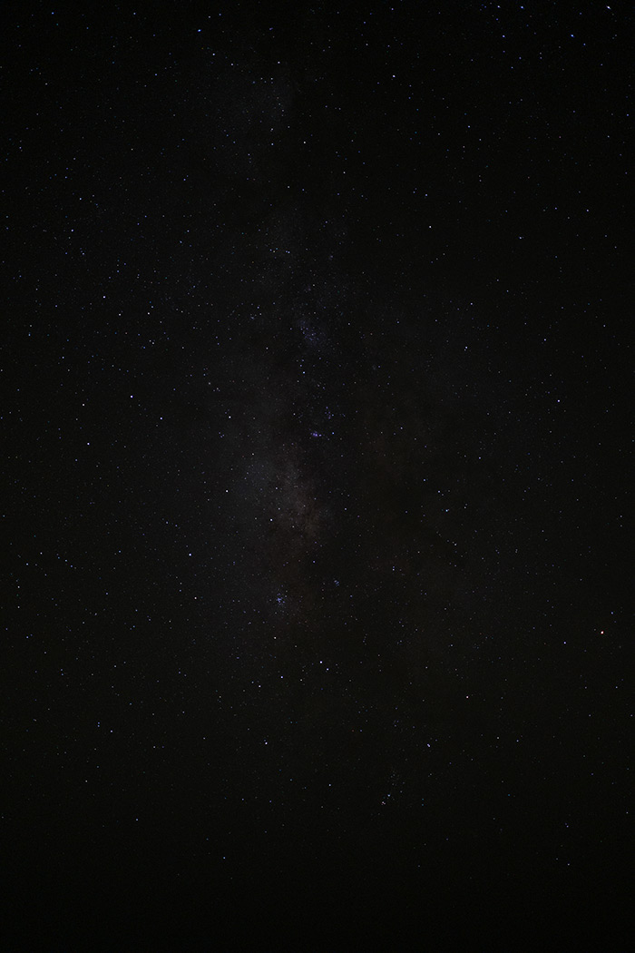
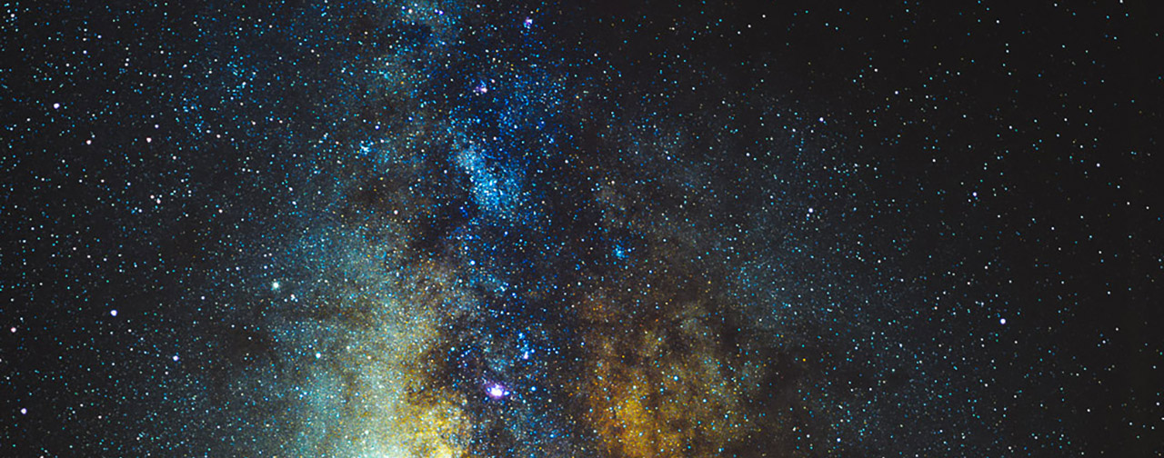
That’s already a nice photo and you can even see the milky-way as the foggy area in the middle of the frame. But if you ever visited a place without any significant light-pollution you probably know, that if you let your eyes adjust to the darkness a little bit you can make out the milky-way just as good. So lets try to boost the brightness of the image a little.
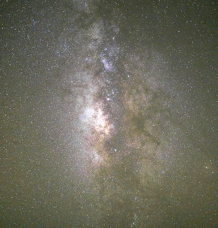
Figure 1: Center-cropped version of the image.
This simple tweak already revealed a lot of previously hidden information i.e. stars. But unfortunately the picture quality also suffered. This is primarily the case, because not only information we want to be visible was revealed, but also the noise that was introduced by the cameras sensor while taking the exposure. Even with naive noise-reduction added during pre-processing, we can’t increase the picture quality without removing significant detail we are interested in.
Another approach to reducing the difference in noise and actual information is to just expose for a longer period of time. If we let the sensor capture more light from the stars we preserve more information in the final image.
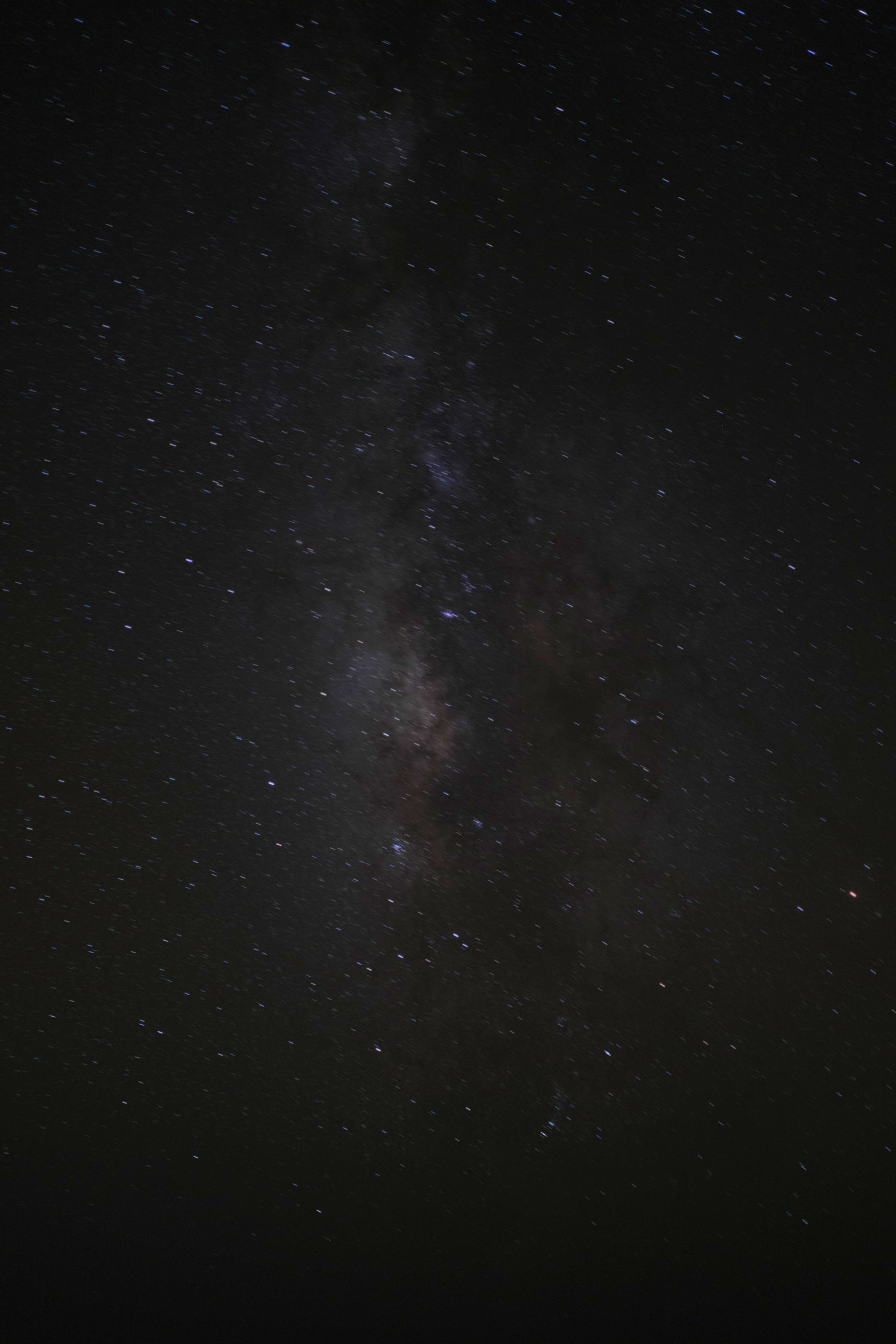
We were successful in capturing more information with a longer exposure. But we didn’t take the rotation of the night-sky into account. This resulted in the stars becoming trails instead of points. To counteract the rotation we could get a tracking camera mount, that will move with the night-sky accordingly. Unfortunately this kind of equipment is quite expensive and cumbersome to carry with. So maybe we shouldn’t give up on a digital solution to our problem just yet. We know a couple hard limits that we can’t overcome:
- Long exposures introduce movement into the frame.
- Increasing the brightness of a frame significantly results in a noisy image.
- Noise levels are to high to remove via post-processing.
The workaround for these limitations is to not only take a single image, but a whole array of them. Each shot with the maximum exposure time while at the same time avoiding star-trails. We can fuse these images together with Exposure or Image Stacking.
Exposure/Image Stacking
Lets say we have a series of image \(I_i\), all taken with a fixed camera position. We can just average every pixel across all images and in return get a single image \(I'\) with less noise. This simple algorithms can be described as \(I'= \sum^c_{i=0} \frac{I_i}{c}\). Lets try it out on a dataset of \(16\) images.
The resulting image is almost exactly the same as the single long exposure we took earlier. We can also see the star-trails clearly, because we forgot to account for the rotation of the night-sky. The only feasible solution would be to revert the rotation digitally. Or in other words rotate the image by an angle \(\alpha\) around a center of rotation \(P\). Unfortunately for us we don’t know \(\alpha\) nor \(P\). Of course we can manually try to find a value for \(\alpha\) and \(P\) that works with our dataset, but we would like to solve our problem entirely programmatical. So no random guessing is necessary by the user. Fortunate for us we can derive the center of rotation \(P\) and \(\alpha\) by finding corresponding stars in two separate frames.
Star Detection
To even start finding correspondence across stars, we need to first identify them as such.
OpenCV already provides a function that allows us to find stars in images: opencv::xfeatures2d::StarDetector.
The
opencvmodulexfeatures2dis non free. And the~opencv::xfeatures2d::StarDetector~is based on: Motilal Agrawal, Kurt Konolige, and Morten Rufus Blas. Censure: Center surround extremas for realtime feature detection and matching. In Computer Vision–ECCV 2008, pages 102–115. Springer, 2008.
If you would like to not use non-free algorithms you can try to create your own keypoint detection algorithm.
Or just use an off-the-shelve general purpose keypoint extractor like SIFT.
For now we are going to stick with the non-free StarDetector.
| |
With the function described above, we retrieve a Vector of KeyPoint s for a given image.
A KeyPoint primarily contains information about the coordinates of a stars and its estimated size.
It’s important to note, that our goal is not to detect all stars in a given image.
We just want enough to later match them against stars in another frame.
Finding Correspondence
Now that we can extract stars out of frames, we can start matching stars of one frame to the same star in another frame. I am going to make the assumption that stars are just moving a couple pixels from one frame to another. We certainly can use an algorithm that works even for examples where there are significant distances between stars in two different pictures, but the assumption will simplify the implementation for now.
The algorithm I am going to be using matches stars that are closest to another in two different frames. So for every star \(P_i\) in the first frame we are measuring the distance to every star \(P'_j\) in the second frame. The distance function we are going to use is the squared distance between two points. \[ dist(x, y) = \sqrt{(P_i - P_j') \cdot (P_i - P_j')} \]
And for a point \(P_i \in I_1\) we are going to pick \(P'_j \in I_2\) that results in the lowest distance: \[ arg\ min_{P'_j}\ dist(P_i, P'_j) \]
To improve the matching algorithm further we can introduce a hyper-parameter \(t\) that describes the maximum distance we are going to allow for a set of two stars. Depending on the interval we shot our stars with we have to increase or decrease the value of \(t\). Generally a lower value for \(t\) will result in a more accurate matching result.
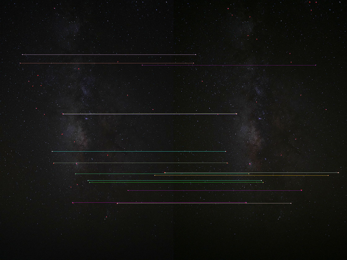
Figure 2: Detected corresponding stars in two distinct images (left/right). Visualization generated with opencv::features2d::draw_matches.
Reversing the Rotation of the Night-Sky
Now that we have a list of star pairs and their pixel coordinates,
we can start working on aligning both images over one another.
We are going to use an affine transformation for this task.
After an affine transformation points in the source image that
form a line still do after the transformation.
To calculate the transformation parameters i.e. rotation, translation and scale,
we can use a homography.
Fortunate for us opencv also supplies us the tools for calculating the
homography matrix, as well as doing the transformation.
| |
First we are going to extract the center-coordinate of each DMatch in our list of matches.
We don’t care about other values like radius and so on.
The opencv::calib3d::find_homography function requires two lists of 2-D coordinates
(Point2f) with corresponding points sharing the same index.
We can leave all other parameters at their default values for now.
Now that we calculated the homography matrix we can apply it to our image(s). First we are going to implement a naive and inefficient way of aligning all images. Lets say we have an ordered series of images \(I_{0..n}\). We are going to align images \(I_{i..n}\) with \(I_{i-1}\), starting with \(i=n\) as long as \(i > 0\). So in the end we are going to end up with a list of images all aligned to \(I_0\). We feed this list into our already existing image averaging function to get a result.
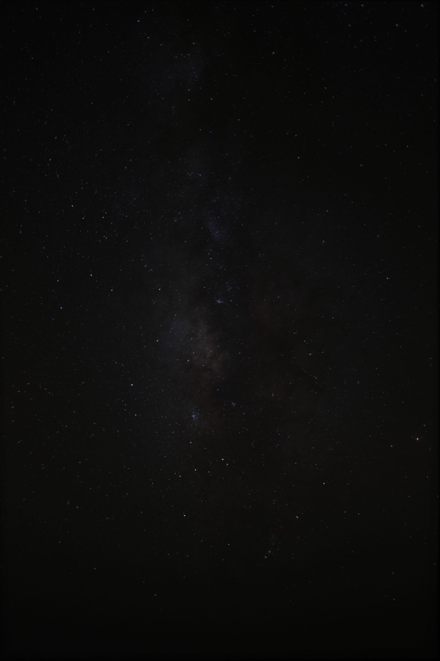
Figure 3: Averaged and aligned image (16 images total)
The image is still quite dark but if we look closely the star-trails disappeared.
Results & Evaluation
To evaluate how much of an improvement the image stacking had we can visualize a single frame with the aligned and averaged image. If we just view them side by side we can’t really tell any real benefit right away, because the noise we want to remove is for the most part hidden in the dark regions of the image. The quality of some regions even decreased without any editing, for example the milky-way looks less defined in the merged image.
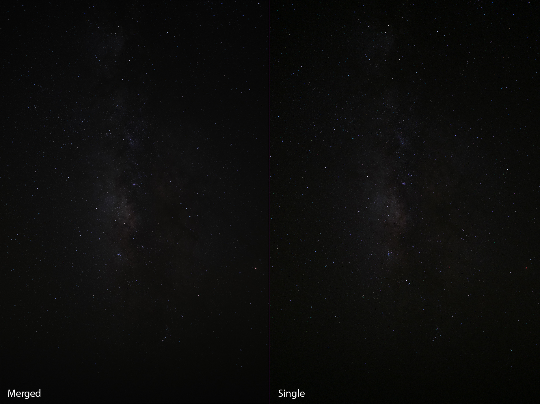
Figure 4: Comparison between a single frame and the merged result image.
Lets increase the brightness of both images equally with a levels adjustment. We can instantly see a difference in both images. Primarily color noise improved a lot of smaller dots got removed. Color gradients look a significantly smoother in darker areas.
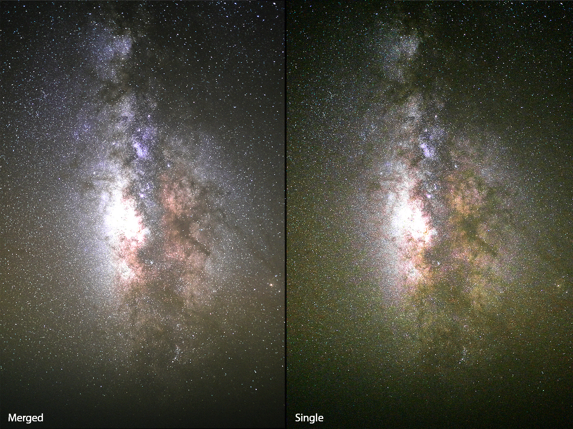
Figure 5: Increasing the brightness of both images equally reveals the achieved noise reduction.
If we zoom into both images we can clearly observe what our algorithm did. You can even still make out that some stars do still have small star-trails. This artifact is introduced into the image because of star detection or matching inaccuracies.
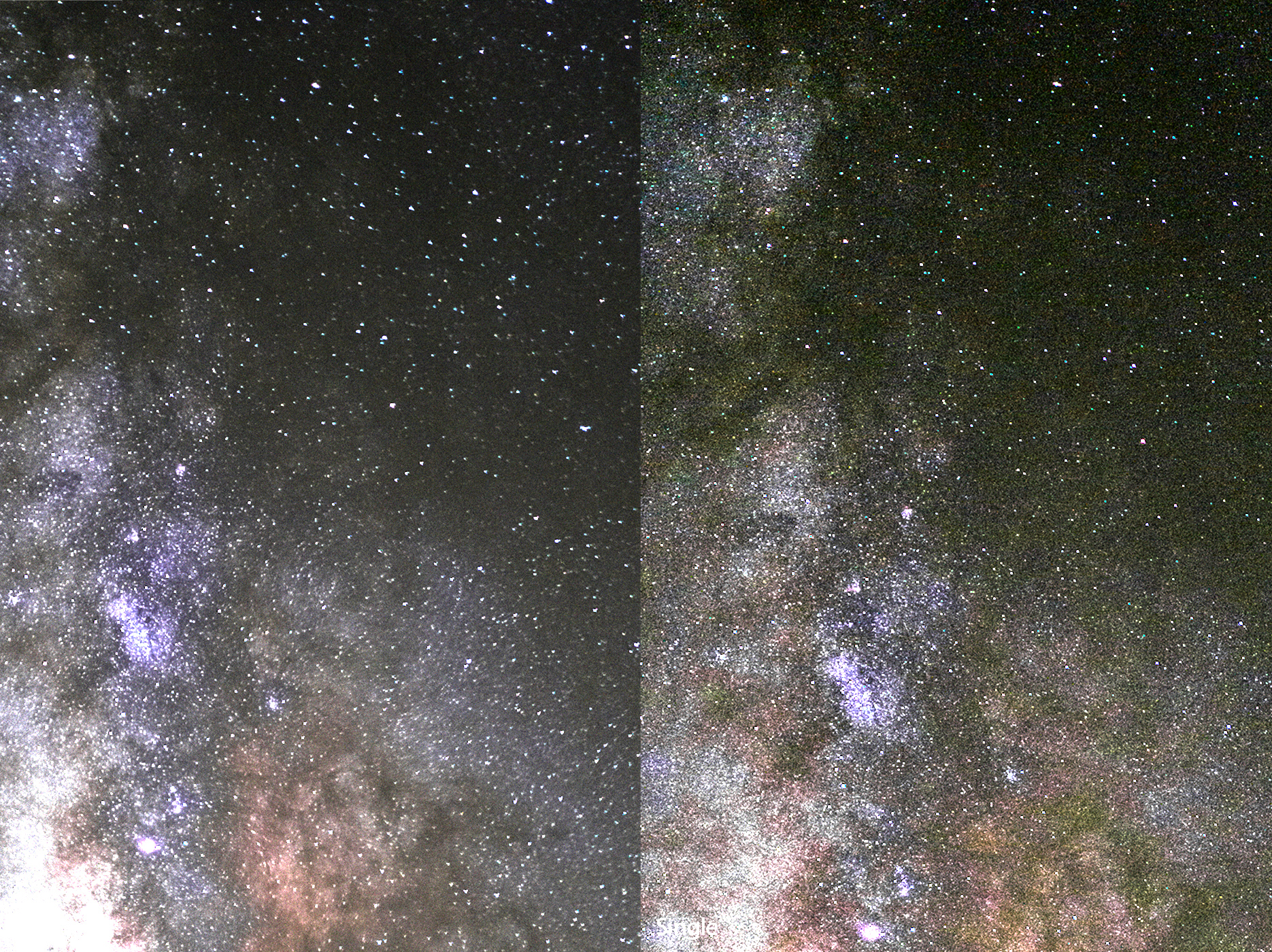
Figure 6: Close-up of roughly the same region of both images.
You can find the code that was used to generate the examples shown in this article, in the GitHub repository linked blow.